[Un po' di nicchia] Rappresentazione spazio-stato e filtro di Kalman

[Cren]

Ho fortunosamente recuperato il listato in R per il tutorial sulla rappresentazione spazio-stato e sull'uso del filtro di Kalman per la stima dei parametri.

L'ho aggiornato e ho modificato i commenti in Inglese in modo da renderlo più vicino all'analisi di dati finanziari.

Rispetto agli esempi di Jouni Helske - che naturalmente ringrazio per essersi preso la briga di scrivere le funzioni usate per la rappresentazione e il filtro - io ho aggiunto l'applicazione allo SPY con relativo trading system fallimentare a dimostrazione che il trend following con una media mobile non è affatto ciò che si pensa che sia.

Sperando di fare cosa gradita (ma questo è veramente di nicchia, temo ), copiate in R e lanciate; nella sezione del back test alcune righe richiedono diversi minuti di elaborazione.

Se lanciate riga per riga anzichè tutto, sicuramente si capisce di più quello che state facendo.

(Mi scuso per eventuali bestialità anglosassoni nei commenti, ma l'assenza di un correttore di ortografia rende molto più probabile che abbia disseminato errori ortografici qua e là).

[COLOR="Teal"]# ================================================================== #
# Kalman filter: a cuttin' edge framework for financial time series? #
# By Cren (and thanks to Jouni Helske for functions)                 #
# ================================================================== #

# Index:

## 1. meeting Kalman filter with examples
## 2. using Kalman filter like a moving average
## 3. rollapplying Kalman filter to see differences with static estimation
## 4. building univariate state-space models
## 5. building multivariate state-space models
## 6. conclusions

# Loading package[/COLOR]

library(ggplot2)
library(gmp)
library(KFAS)
library(quantmod)
library(PerformanceAnalytics)

[COLOR="teal"]## 1. meeting Kalman filter with examples

# Example of local level model for Nile series[/COLOR]

y <- Nile
qplot(y = y, x = index(y), geom = 'line', ylab = 'Nile', xlab = 'Year')

[COLOR="teal"]# Function 'structSSM' creates a state space representation of structural time
# series[/COLOR]

modelNile <- structSSM(y = y)

[COLOR="teal"]# Function 'fitSSM' finds the maximum likelihood estimates for unknown 
# parameters of an arbitary state space model if an user defined model building 
# function is defined. As a default, 'fitSSM' estimates the non-zero elements, 
# which are marked as NA, of the time-invariant covariance matrices H and Q of
# the given model.[/COLOR]

fit <- fitSSM(inits = c(0.5 * log(var(Nile)), 0.5 * log(var(Nile))), 
              model = modelNile)

[COLOR="teal"]# Filtering and state smoothing: performs Kalman filtering and smoothing with
# exact diffuse initialization using univariate approach for exponential family
# state space models. For non-Gaussian models, state smoothing is provided with
# additional smoothed mean and variance of observations[/COLOR]

kfsNile <- KFS(fit$model, smoothing = 'state')

[COLOR="teal"]# Simple plot of series and the smoothed 'signal = Z * alpha_hat'[/COLOR]

plot(kfsNile, col = 1:2, lwd = 1:2) ; grid()

[COLOR="teal"]# Confidence intervals for the state[/COLOR]

lows <- c(kfsNile$alphahat - qnorm(0.95) * sqrt(c(kfsNile$V)))
ups <- c(kfsNile$alphahat + qnorm(0.95) * sqrt(c(kfsNile$V)))
plot.ts(cbind(y, c(kfsNile$alphahat), lows, ups), plot.type = 'single', 
        col = c(1:2, 3, 3), ylab = 'Predicted annual flow', main = 'River Nile',
        lwd = c(1, 2, 2, 2)) ; grid()

[COLOR="teal"]# Example of multivariate local level model with only one state
# Two series of average global temperature deviations for years[/COLOR]

data(GlobalTemp)

[COLOR="teal"]# Function 'SSModel' creates a state space object of class 'SSModel' which 
# can be used as an input object for various functions of KFAS package[/COLOR]

modelTemp <- SSModel(y = GlobalTemp, Z = matrix(1, nrow = 2), T = 1, R = 1, 
                     H = matrix(NA, 2, 2), Q = NA, a1 = 0, P1 = 0, P1inf = 1)

[COLOR="teal"]# Estimating the variance parameters[/COLOR]

fit <- fitSSM(inits = c(0.5 * log(.1), 0.5 * log(.1), 0.5 * log(.1), 0), 
              model = modelTemp)
outTemp <- KFS(fit$model, smooth = 'both')
ts.plot(cbind(modelTemp$y, t(outTemp$alphahat)), col = 1:3, 
        lwd = c(1, 1, 2)) ; grid()
legend('bottomright',legend = c(colnames(GlobalTemp), 'Smoothed signal'), 
       col = 1:3, lty = 1, lwd = c(1, 1, 2))

[COLOR="teal"]# Example of multivariate series where first series follows stationary ARMA(1,1)
# process and second stationary AR(1) process
[/COLOR]
y1 <- arima.sim(model = list(ar = 0.8, ma = 0.3), n = 100, sd = 0.5)

[COLOR="teal"]# Function 'arimaSSM' creates a state space representation of ARIMA model[/COLOR]

model1 <- arimaSSM(y = y1, arima = list(ar = 0.8, ma = 0.3), Q = 0.5 ^ 2)
y2 <- arima.sim(model = list(ar = -0.5), n = 100)
model2 <- arimaSSM(y = y2, arima = list(ar = -0.5))
model <- model1 + model2
f.out <- KFS(model)
         
[COLOR="teal"]# Drivers[/COLOR]

Seatbelts
model <- structSSM(y = log(Seatbelts[,'drivers']), trend = 'level', 
                   seasonal = 'time', X = cbind(log(Seatbelts[,'kms']),
                                                log(Seatbelts[,'PetrolPrice']),
                                                Seatbelts[, c('law')]))
fit <- fitSSM(inits = rep(-1, 3), model = model)
out <- KFS(fit$model, smoothing = 'state')
plot(out, lty = 1:2, col = 1:2, main = '')

[COLOR="teal"]# Function 'signal' extracts the filtered or smoothed signal of a State Space 
# model depending on the input object
[/COLOR]
lines(signal(out, states = c(1, 13:15))$s, col = 4, lty = 1)
legend('bottomleft', legend = c('Observations', 'Smoothed signal', 
                                'Smoothed level'), col = c(1, 2, 4),
       lty = c(1, 2, 1))

[COLOR="teal"]# Multivariate model with constant seasonal pattern in frequency domain[/COLOR]

model <- structSSM(y = log(Seatbelts[,c('front', 'rear')]), trend = 'level',
                   seasonal = 'freq', X = cbind(log(Seatbelts[,c('kms')]),
                                                log(Seatbelts[,'PetrolPrice']),
                                                Seatbelts[,'law']), H = NA,
                   Q.level = NA, Q.seasonal = 0)
sbFit <- fitSSM(inits = rep(-1, 6), model = model)
out <- KFS(sbFit$model, smoothing = 'state')
ts.plot(signal(out, states = c(1:2, 25:30))$s, model$y, col = 1:4)

[COLOR="teal"]# What have we learnt so far?

# a. We can use either 'SSModel' and 'structSSM' to build up a state-space 
# model;
# b. 'fitSSM' allows us to estimate maximum likelihood variance of the model
# c. 'KFS' performs the Kalman filter
# d. 'signal' extracts the filtered or smoothed signal of a State Space 
# model depending on the input object

## 2. using Kalman filter like a moving average[/COLOR]

getSymbols('SPY', from = '1950-01-01', src = 'yahoo')
obs <- SPY
y <- log(Cl(to.daily(obs)))
chartSeries(y)

[COLOR="teal"]# State-space model:
# y(t) = Z * alpha(t) + e(t), e(t) ~ N(0, H(t))
# alpha(t + 1) = T * alpha(t) + R(t) * h(t), h(t) ~ N(0, Q(t))[/COLOR]

model <- SSModel(y = as.ts(y), Z = 1, T = 1, H = 1, Q = 1)
[COLOR="teal"]#fit <- fitSSM(inits = rep(0.5 * log(.1), 2), model = model)[/COLOR]
out <- KFS(object = model, smoothing = 'state')
plot(out, col = 1:2) ; grid()

[COLOR="teal"]# Note that using MLE fit on a in-sample financial time series may return a
# perfect fit, which is not the result we would like to get. By the way,
# there's no difference in using specific diagonal variance matrices elements
# unless these variables are set equal to NULL or MLE parameters

## 3. rollapplying Kalman filter to see differences with static estimation

# Kalman filter smoothing function with MLE

# State-space model:
# y(t) = Z * alpha(t) + e(t), e(t) ~ N(0, H(t))
# alpha(t + 1) = T * alpha(t) + R(t) * h(t), h(t) ~ N(0, Q(t))[/COLOR]

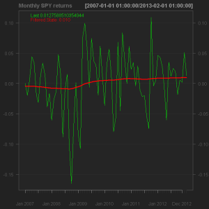
ks <- function(y){
  y <- Cl(to.monthly(y))
  y <- log(as.ts(y))
  model <- SSModel(y = y, Z = 1, T = 1, H = NA, Q = NA)
  fit <- fitSSM(inits = rep(0.5 * log(.1), 2), model = model)
  out <- KFS(object = fit$model, smoothing = 'state')
  return(exp(tail(t(out$alphahat), 1)))
}

KFMA <- rollapplyr(data = Cl(obs), width = 252 * 2, FUN = ks)
plot.xts(SPY, log = 'y')
lines(KFMA, col = 2, lwd = 1)

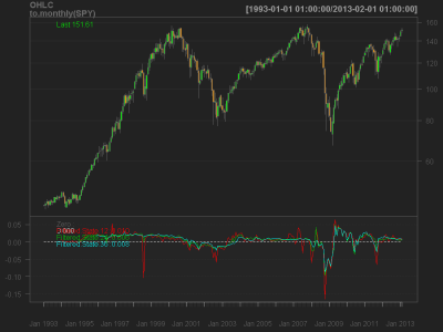
[COLOR="teal"]# A small variation: LOESS featuring Kalman filter

# State-space model:
# y(t) = Z * alpha(t) + e(t), e(t) ~ N(0, H(t))
# alpha(t + 1) = T * alpha(t) + R(t) * h(t), h(t) ~ N(0, Q(t))
# Here y(t) is the LOESS value[/COLOR]

lks <- function(y, span){
  y <- log(y)
  x <- 1:length(y)
  loess <- loess(formula = y ~ x, span = span)
  y <- as.ts(loess$fitted)
  model <- SSModel(y = y, Z = 1, T = 1, H = NA, Q = NA)
  fit <- fitSSM(inits = rep(0.5 * log(.1), 2), model = model)
  out <- KFS(object = fit$model, smoothing = 'state')
  return(exp(mean(tail(t(out$alphahat), 5))))
}

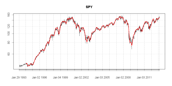
KFMA <- rollapplyr(data = Cl(obs), width = 252, FUN = lks, span = .95)
plot.xts(SPY, log = 'y', lty = 2)
lines(KFMA, col = 2, lwd = 2)
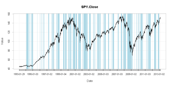
trig <- ifelse(KFMA >= lag(KFMA), 1, 0)
per.ar.0 <- index(trig[trig != lag(trig)])

if(is.whole(length(per.ar.0) / 2) == FALSE){
  per.ar <- c(per.ar.0, index(tail(KFMA, 1)))
} else{
  per.ar <- per.ar.0
}

period.areas <- NULL

for(i in seq(1, length(per.ar), 2)){
  period.areas[i] <- paste(per.ar[i], per.ar[i + 1], sep = '/')
}

period.areas <- na.omit(period.areas)

chart.TimeSeries(R = Cl(obs), log = 'y', period.areas = period.areas,
                 period.color = 'lightblue', lwd = 1)

[COLOR="teal"]# Equity line of basic trading system[/COLOR]

ret.cc <- ClCl(obs)
ret.oc <- OpCl(obs)
ret <- lag(trig) * ifelse(lag(trig) != lag(trig, 2), ret.oc, ret.cc)
charts.PerformanceSummary(R = ret)

[COLOR="teal"]# This shows you cannot really use a low-pass filter to trade prices because of
# unavoidable lag, while Kalman filter cannot "see" trend components beyond
# noise more than a simple moving average can do

## 4. building univariate state-space models

# Summary (again):

# a. We can use either 'SSModel' and 'structSSM' to build up a state-space 
# model;
# b. 'fitSSM' allows us to estimate maximum likelihood variance of the model
# c. 'KFS' performs the Kalman filter
# d. 'signal' extracts the filtered or smoothed signal of a State Space 
# model depending on the input object

# State-space model:
# y(t) = Z * Alpha(t) + E(t), E(t) ~ N(0, H(t))
# Alpha(t + 1) = T * Alpha(t) + R(t) * H(t), H(t) ~ N(0, Q(t))
# Hence Alpha, E and H are matrices[/COLOR]

[COLOR="teal"]# We've already seen the 'Seatbelts' data frame: how have 'PetrolPrice' and
# 'law' affected 'DriversKilled' over time?
[/COLOR]
(Seatbelts)
model <- structSSM(y = log(Seatbelts[,'DriversKilled']), 
                   X = cbind(log(Seatbelts[,'PetrolPrice']), 
                             Seatbelts[,'law']), H = NA, Q.level = NA)
fit <- fitSSM(inits = rep(.5 * log(.1), 2), model = model)
out <- KFS(object = fit$model, smoothing = 'state')
Beta <- matrix(NA, nrow = nrow(Seatbelts), ncol = 3)

for(i in 1:3){
  Beta[,i] <- signal(out, i)$signal
}

colnames(Beta) <- c('Intercept', 'Beta 1', 'Beta 2')
plot.zoo(Beta, xaxt = 'n', xlab = '')

[COLOR="teal"]## 5. building multivariate state-space models

# State-space model:
# Y(t) = Z * Alpha(t) + E(t), E(t) ~ N(0, H(t))
# Alpha(t + 1) = T * Alpha(t) + R(t) * H(t), H(t) ~ N(0, Q(t))
# Hence Y, Alpha, E and H are matrices[/COLOR]

Seatbelts
model <- structSSM(y = cbind(log(Seatbelts[,'DriversKilled']),
                             log(Seatbelts[,'drivers'])),
                   X = cbind(log(Seatbelts[,'PetrolPrice']), 
                             Seatbelts[,'law']))
fit <- fitSSM(inits = rep(.5 * log(.1), 4), model = model)
out <- KFS(object = fit$model, smoothing = 'state')

[COLOR="teal"]# Checking differences between filtered states and OLS regression coefficients
[/COLOR]
Y <- cbind(log(Seatbelts[,'DriversKilled']), log(Seatbelts[,'drivers']))
X <- cbind(log(Seatbelts[,'PetrolPrice']), Seatbelts[,'law'])
summary(lm(Y ~ X))
plot(signal(object = out, states = 3:4)$signal, main = '')

[COLOR="teal"]## 6. conclusions

# What have we learnt about state - space models and Kalman filter?
# State - space representation is suitable to describe linear models, like
# structural time series and linear regressions. State - space model time 
# varying parameters can be estimated via Kalman filter: maximum likelihood is
# used to get residuals covariance matrices, and a smoothed state signal can be
# obtained.

# What Kalman filtered state - space represention CANNOT do: to extract a trend
# component which could be "followed" to gain profits from financial 
# instruments' time series.

# What Kalman filtered state - space represention CAN do: to model every 
# linear relation out there regardless of time series sample dimensions; every
# time series analysis practitioner has always found difficulties in sampling
# financial time series to perform parameters estimation, that is why expanding
# and/or rolling window are broadly used.[/COLOR]

 

[Key West]

Applicato il KF sui prezzi dello SP500?

Uhmm...e perchè?

 

[Cren]

Applicato il KF sui prezzi dello SP500?

No.

 

[Key West]

No.

Chiedo scusa, ero convinto che nel tuo esempio avessi usato i logprezzi sostituendo il filtro ad una semplice MA su di essi.

Ho vsto male, scusa ancora.

 

[Cren]

Uhmm...e perchè?

Se comprendo la tua (eventuale) osservazione, tu ti riferisci a questa applicazione del filtro di Kalman, cioè la variabile di stato come intercetta di un modello spazio-stato sui rendimenti.

Ho compreso bene dove vuoi arrivare?

 

[Key West]

Se comprendo la tua (eventuale) osservazione, tu ti riferisci a questa applicazione del filtro di Kalman, cioè la variabile di stato come intercetta di un modello strutturale sui rendimenti.

Ho compreso bene dove vuoi arrivare?

Sì.

Mi spiace di essermi rin********to, ho letto di sfuggita e guardato di sfuggita e ripeto, ero convintssimo tu avessi fatto un esempio del filtro dei logprezzi dello SPY.

Chiedo scusa again..

 

[Cren]

Chiedo scusa, ero convinto che nel tuo esempio avessi usato i logprezzi sostituendo il filtro ad una semplice MA su di essi.

No, in input è stato usato il trend ricavato da regressione locale sul tempo (il procedimento è analogo alla decomposizione STL delle serie storiche) e successivamente questo è stato elaborato come modello strutturale di cui stimare i parametri col filtro.

So che sembra una complicazione enorme, ma - se fai andare il listato - vedi che c'è anche la parte che dici tu... e vedi che usare così (cioè: come una media mobile) il filtro è inutile (da cui credo derivino i dubbi del tuo primo messaggio).

L'ho messa apposta perchè è una delle prime cose che di solito si vuol fare quando si approccia il modello spazio-stato.

 

[Key West]

No, in input è stato usato il trend ricavato da regressione locale sul tempo (il procedimento è analogo alla decomposizione STL delle serie storiche) e successivamente questo è stato elaborato come modello strutturale di cui stimare i parametri col filtro.

So che sembra una complicazione enorme, ma - se fai andare il listato - vedi che c'è anche la parte che dici tu... e vedi che usare così (cioè: come una media mobile) il filtro è inutile (da cui credo derivino i dubbi del tuo primo messaggio).

L'ho messa apposta perchè è una delle prime cose che di solito si vuol fare quando si approccia il modello spazio-stato.

Esatto...meno male che non sono allora del tutto rin********to...

Io capisco che l'hai messa apposta ma..la mia domanda è:

che senso ha applicare una predizione sui logprezzi? (ricordiamoci come è costituito un KF...)

Vado in palestra che me sto a fa er fisico..quando torno leggo..

ps: c'è una tesi del Politecnico sul KF applicato al Pairs Trading..guarda se hai l'accesso ancora..

 

[Cren]

L'applicazione "corretta" del modello spazio-stato e del filtro di Kalman è quella che faccio nei punti 4. e 5., cioè: hai un modello lineare, come una regressione, che mette in relazione il numero di morti alla guida con i prezzi della benzina e l'introduzione di una legge sulle cinture di sicurezza.

Se usi gli OLS, trovi i parametri della regressione per il tuo campione.

Ma siamo sicuri che questi valori vadano bene per tutto il campione (cioè che siano costanti)?

No, e quindi procediamo alla stima dei parametri col filtro di Kalman: osserviamo che infatti il coefficiente associato a una legge sulle cinture di sicurezza non vale nulla fino all'introduzione della legge stessa (il coefficiente è zero), dopodichè ha un impatto non marginale sui morti per incidenti stradali (a memoria mi sembra -0.20 sul logaritmo naturale dei morti).

Questo è un esempio stupido perchè la variabile è una dummy, ma era l'unico che non richiedeva ragionamento logico; interessante vedere l'impatto nel corso del tempo, ad esempio, del prezzo della benzina.

che senso ha applicare una predizione sui logprezzi? (ricordiamoci come è costituito un KF...)

Pagina 14 di questa presentazione (che non avevo allegato a caso): una serie storica può essere rappresentata come componente deterministica e componente stocastica (nessuna novità qui), ma la rappresentazione spazio-stato consente in teoria di ricavare - in soldoni - «come il prezzo di ieri influenza il prezzo di oggi» assumendo anche stagionalità mediante l'evoluzione della variabile di stato.

So che esistono dei programmi di analisi tecnica & affini che mettono "filtro di Kalman" tra le medie mobili usando questa rappresentazione & smussandola un po': per le serie finanziarie di prezzi non funziona, è solo un espediente commerciale

Nell'esempio si vede bene la differenza con il livello del Nilo e lo SPY: benché entrambe possano essere descritte con un semplice modello strutturale pressoché identico, il fit dello SPY non produce per nulla il comodo "smooth" del Nilo.

 

[Key West]

L'applicazione "corretta" del modello spazio-stato e del filtro di Kalman è quella che faccio nei punti 4. e 5., cioè: hai un modello lineare, come una regressione, che mette in relazione il numero di morti alla guida con i prezzi della benzina e l'introduzione di una legge sulle cinture di sicurezza.

Se usi gli OLS, trovi i parametri della regressione per il tuo campione.

Ma siamo sicuri che questi valori vadano bene per tutto il campione (cioè che siano costanti)?

No, e quindi procediamo alla stima dei parametri col filtro di Kalman: osserviamo che infatti il coefficiente associato a una legge sulle cinture di sicurezza non vale nulla fino all'introduzione della legge stessa (il coefficiente è zero), dopodichè ha un impatto non marginale sui morti per incidenti stradali (a memoria mi sembra -0.20 sul logaritmo naturale dei morti).

Questo è un esempio stupido perchè la variabile è una dummy, ma era l'unico che non richiedeva ragionamento logico; interessante vedere l'impatto nel corso del tempo, ad esempio, del prezzo della benzina.

Pagina 14 di questa presentazione (che non avevo allegato a caso): una serie storica può essere rappresentata come componente deterministica e componente stocastica (nessuna novità qui), ma la rappresentazione spazio-stato consente in teoria di ricavare - in soldoni - «come il prezzo di ieri influenza il prezzo di oggi» assumendo anche stagionalità mediante l'evoluzione della variabile di stato.

So che esistono dei programmi di analisi tecnica & affini che mettono "filtro di Kalman" tra le medie mobili usando questa rappresentazione & smussandola un po': per le serie finanziarie di prezzi non funziona, è solo un espediente commerciale

Nell'esempio si vede bene la differenza con il livello del Nilo e lo SPY: benché entrambe possano essere descritte con un semplice modello strutturale pressoché identico, il fit dello SPY non produce per nulla il comodo "smooth" del Nilo.

Perchè sono due cose diverse (livelli del nilo e prezzi dello SPY)

E' questo che intendo..non trovo l'esempio corretto perchè il filtro Kalman non ha senso sui prezzi dello SPY. Non so se mi sono spiegato (disse il paracadute).

 

[Cren]

Perchè sono due cose diverse (livelli del nilo e prezzi dello SPY)

E' questo che intendo..non trovo l'esempio corretto perchè il filtro Kalman non ha senso sui prezzi dello SPY.

L'applicazione "corretta" del filtro di Kalman è nella stima dei parametri di un modello ARMA(p,q) mediante massima verosimiglianza, poichè non si conosce a priori qual è la forma della distribuzione condizionata dei residui

Anche questa è una storia vecchia e risaputa: oggi tutti i programmi di analisi delle serie storiche in circolazione usano il filtro di Kalman per la stima di massima verosimiglianza esatta.

Meno scontato è sottolineare che fare il fit sulla serie storica per stimare la covarianza dei residui dà luogo a "sguardi al futuro" molto pericolosi; se non si vuole dare sguardi al futuro, bisogna procedere come ho allegato in immagine.

Nel modello ho cercato di stimare il rendimento mensile dello SPY con filtro di Kalman [il modello spazio-stato è semplice: in pratica è un AR(1)].

L'effetto collaterale si vede subito: l'output che non usa i dati futuri per il fit è dipendente dalla finestra usata (12, 24 e 36 mesi come indicato in legenda)... e si perde rovinosamente ogni smoothing.